This one seems to be straight forward, but there is no flag to be found! Sample rate = 1024k
We are given a single file challenge.cfile. Based on the extension and the mention of sample rate, this is probably a raw software-defined radio recording: a binary file containing complex-valued received samples.
Let’s try to load the file and see what the contents are. I used Matlab:
fd = fopen("challenge.cfile", "r", "ieee-le");
raw = fread(fd, "float32");
s = raw(1:2:end) + 1j*raw(2:2:end);
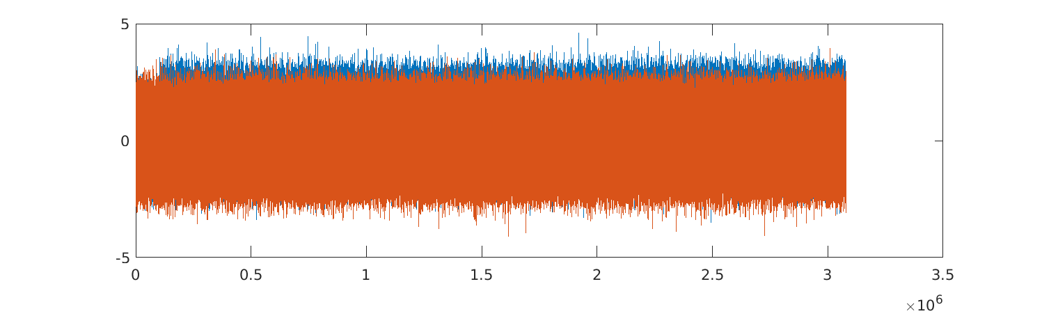
plot(1:length(s), real(s), 1:length(s), imag(s));
From the signal plot, we can see that the file is definitely an SDR recording – if we got the format wrong, we wouldn’t have such a consistent range of values in the input. The real part looks offset, so let’s make the input zero-centered:
s = s - mean(s);Next, I tried a few things to identify the contents of the signal. The Fourier transform is usually a good place to start, since the carrier frequency will show up as an obvious peak if the signal is not transmitted at the same frequency the SDR is tuned to (which would show up as zero). This was not so useful for this challenge, and plotting the autocorrelation of the input was a faster way to the solution:
plot(abs(xcorr(s)));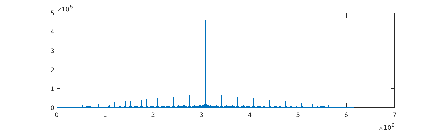
The large peak in the middle will exist for any input, since it corresponds to the zero offset. The other equally-spaced peaks are more interesting – they suggest that the input signal is periodic, probably because the same transmission repeats multiple times. The gap between peaks is 110800, meaning that the transmission repeats every 110800 samples.
We can now split the input into blocks with length B and average them to reduce the noise. This is a naive approach that will not work for real signals, but does work very well for artificial CTF inputs – in real life, the blocks will be out of phase due to oscillator inaccuracies, and averaging them will not improve signal quality.
B = 110800;
nB = floor(length(s) / B);  % number of blocks
s_avg = sum(reshape(s(1:B*nB), [B nB]), 2)';
If we plot this and zoom in, we will see that the real part contains an obvious amplitude-modulated signal:
plot(1:length(s_avg), real(s_avg), 1:length(s_avg), imag(s_avg))
xlim([10000 11000])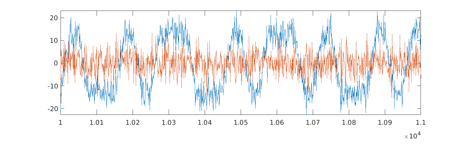
From the plot, we can see that the symbols are 50 samples long and are offset by 15. We can use this to average the signal in each symbol and remove some noise:
L = 50;
off = 15;
nL = floor(length(s_avg)/L) - 1;
s_sym = sum(reshape(real(s_avg(off:off+L*nL-1)), [L nL]));
stairs(s_sym);
xlim([200 220]);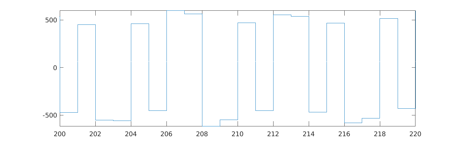
There are at most two consecutive equal symbols, which suggests that the data is Manchester-encoded, using 01 and 10 to represent the zero-bit and one-bit. The quickest way to turn this into decoded data, for me, was to print it and write a bit of Python to replace the 01 and 10 with 0 and 1, and parse as bytes. To get the data out of Matlab:
fprintf("%d", rx > 0);The transmission contents areI've started the transfer (sample rate = 1024k). The chip sequence is: [...], where the [...] is a sequence of bits. We didn’t get a flag, but now we know that there is a secondary transmission using a chip sequence, meaning that it is a spread-spectrum transmission. The chip sequence is transmitted directly to represent 1, and inverted (i.e. multiplied by -1) to represent 0.
To check the length of the chip sequence (so that we don’t accidentally decode noise after the transmission), we can take a part of it and look at the correlation with the input – the gap between peaks will be the length of the chip sequence.
chip = [1 0 0 0 ...];  % 100 bits
chip = 2*chip - 1;  % convert to +1 / -1
plot(abs(xcorr(s, chip)));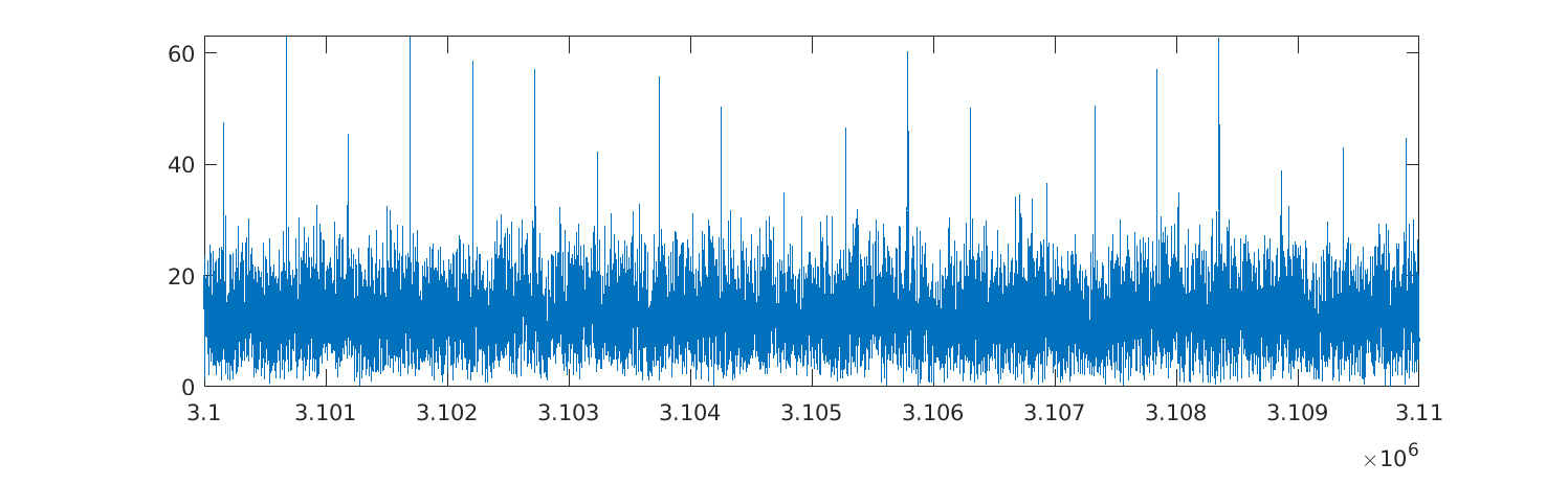
We can see that the chip sequence is 512 bits long, so we can grab the 512 bits after the transmitted message. From the position of the peaks (offsets at which the chip sequence repeats), we know that it starts from the first sample in the input. We can now multiply the input with the chipping sequence to get the demodulated signal (and average each 512-bit long block containing a single symbol):
C = 512;
nC = floor(length(s_avg) / C);
out = s(1:C*nC)' .* repmat(chip, [1 nC]);
out = sum(reshape(out, [C nC]));
plot(1:length(out), real(out), 1:length(out), imag(out))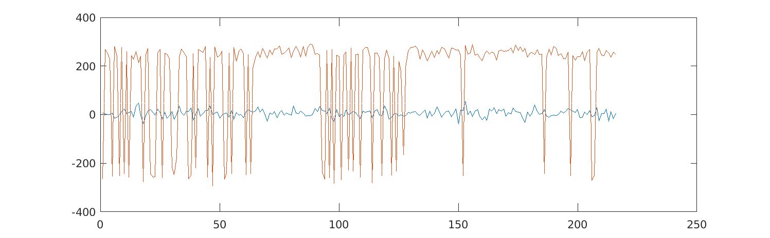
The data is entirely in the imaginary part of the signal, so we can turn it into bits by taking the imaginary part and mapping positive values to 1, and negative ones to -1. We can once again get this out of Matlab by printing:
fprintf("%d", imag(out) > 0);After turning the bit sequence into a file, we get a PNG image containing the flag:
